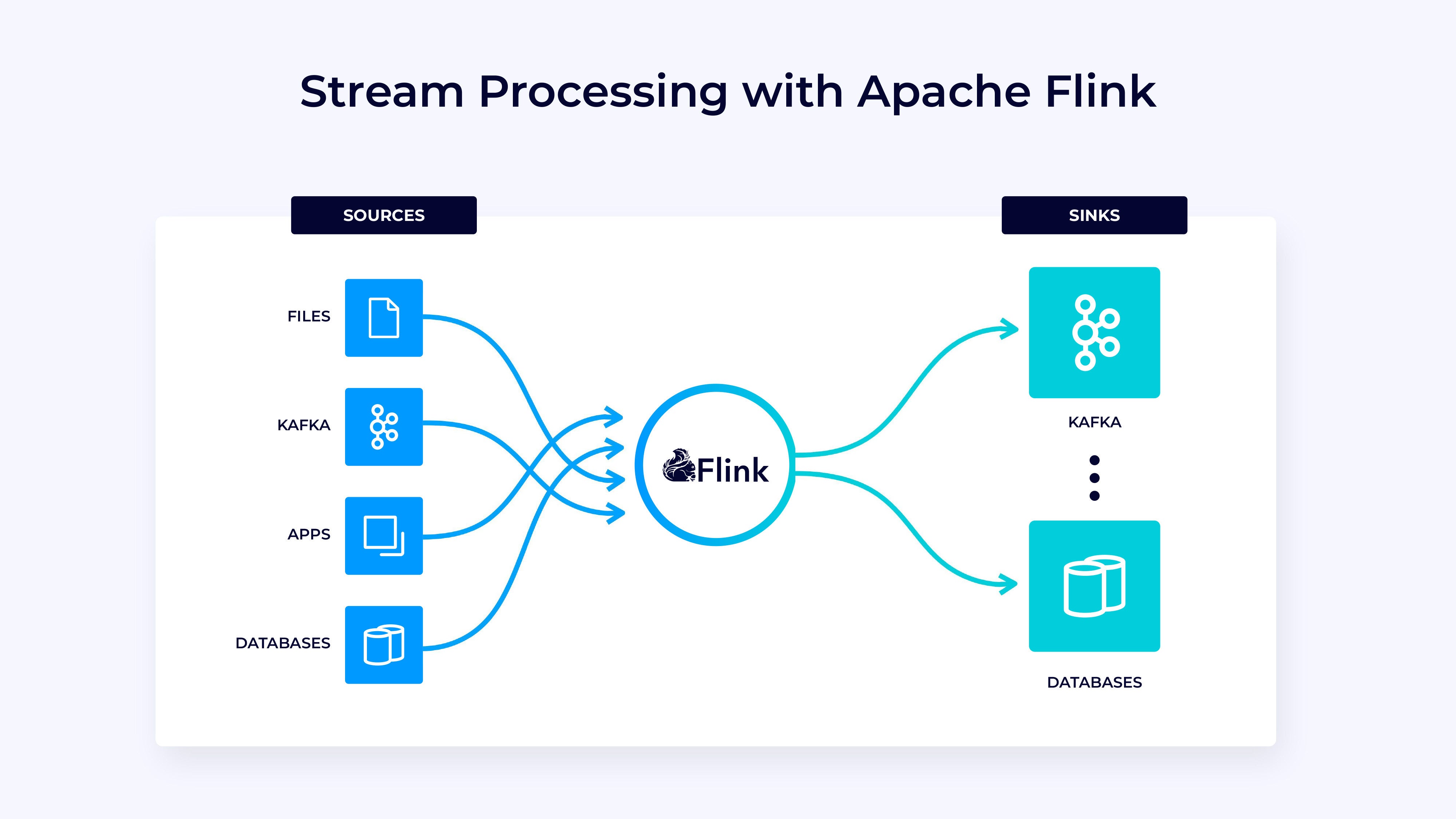
In recent years, Apache Flink has established itself as the de facto standard for real-time stream processing. Stream processing is a paradigm for system building that treats event streams (sequences of events in time) as its most essential building block. A stream processor, such as Flink, consumes input streams produced by event sources, and produces output streams that are consumed by sinks. The sinks store results and make them available for further processing.
Household names like Amazon, Netflix, and Uber rely on Flink to power data pipelines running at tremendous scale at the heart of their businesses. But Flink also plays a key role in many smaller companies with similar requirements for being able to react quickly to critical business events.
IDG
What is Flink being used for? Common use cases fall into three categories.
Streaming data pipelines
Real-time analytics
Event-driven applications
Continuously ingest, enrich, and transform data streams, loading them into destination systems for timely action (vs. batch processing).
Continuously produce and update results which are displayed and delivered to users as real-time data streams are consumed.
Recognize patterns and react to incoming events by triggering computations, state updates, or external actions.
Some examples include:
Streaming ETL
Data lake ingestion
Machine learning pipelines
Some examples include:
Ad campaign performance
Usage metering and billing
Network monitoring
Feature engineering
Some examples include:
Fraud detection
Business process monitoring and automation
Geo-fencing
And what makes Flink special?
Robust support for data streaming workloads at the scale needed by global enterprises.
Strong guarantees of exactly-once correctness and failure recovery.
Support for Java, Python, and SQL, with unified support for both batch and stream processing.
Flink is a mature open-source project from the Apache Software Foundation and has a very active and supportive community.
Flink is sometimes described as being complex and difficult to learn. Yes, the implementation of Flink’s runtime is complex, but that shouldn’t be surprising, as it solves some difficult problems. Flink APIs can be somewhat challenging to learn, but this has more to do with the concepts and organizing principles being unfamiliar than with any inherent complexity.
Flink may be different from anything you’ve used before, but in many respects it’s actually rather simple. At some point, as you become more familiar with the way that Flink is put together, and the issues that its runtime must address, the details of Flink’s APIs should begin to strike you as being the obvious consequences of a few key principles, rather than a collection of arcane details you should memorize.
This article aims to make the Flink learning journey much easier, by laying out the core principles underlying its design.
Flink embodies a few big ideas
Streams
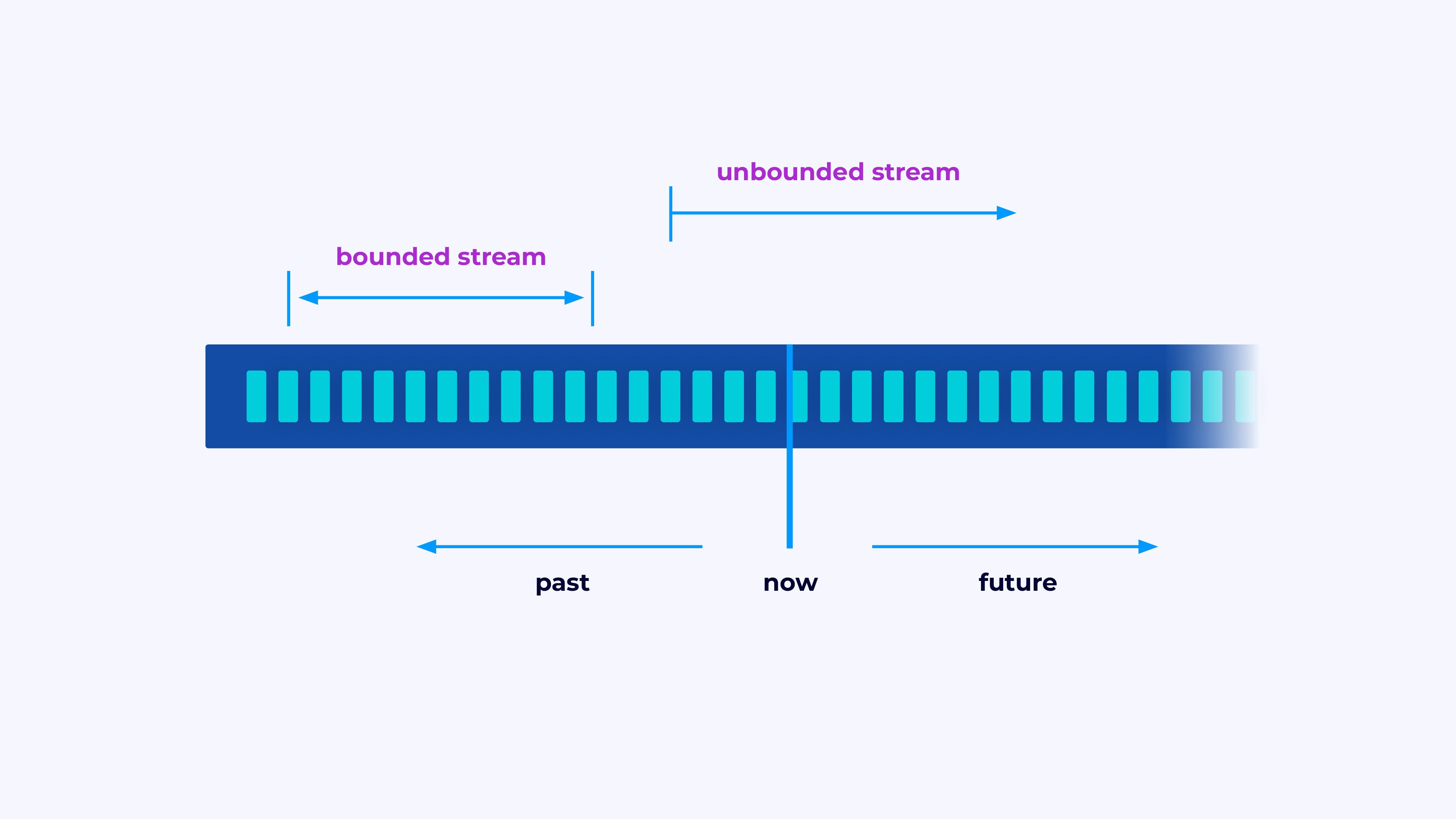
Flink is a framework for building applications that process event streams, where a stream is a bounded or unbounded sequence of events.
IDG
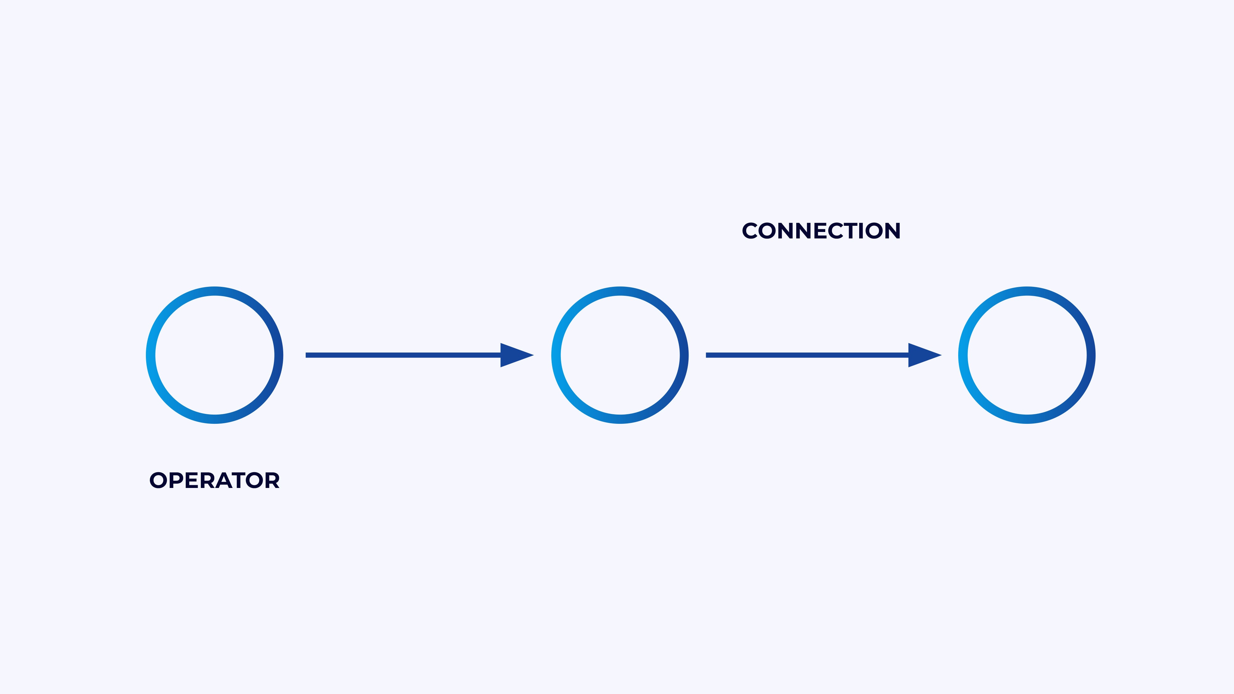
A Flink application is a data processing pipeline. Your events flow through this pipeline, and they are operated on at each stage by code you write. We call this pipeline the job graph, and the nodes of this graph (or in other words, the stages of the processing pipeline) are called operators.
IDG
The code you write using one of Flink’s APIs describes the job graph, including the behavior of the operators and their connections.
Parallel processing
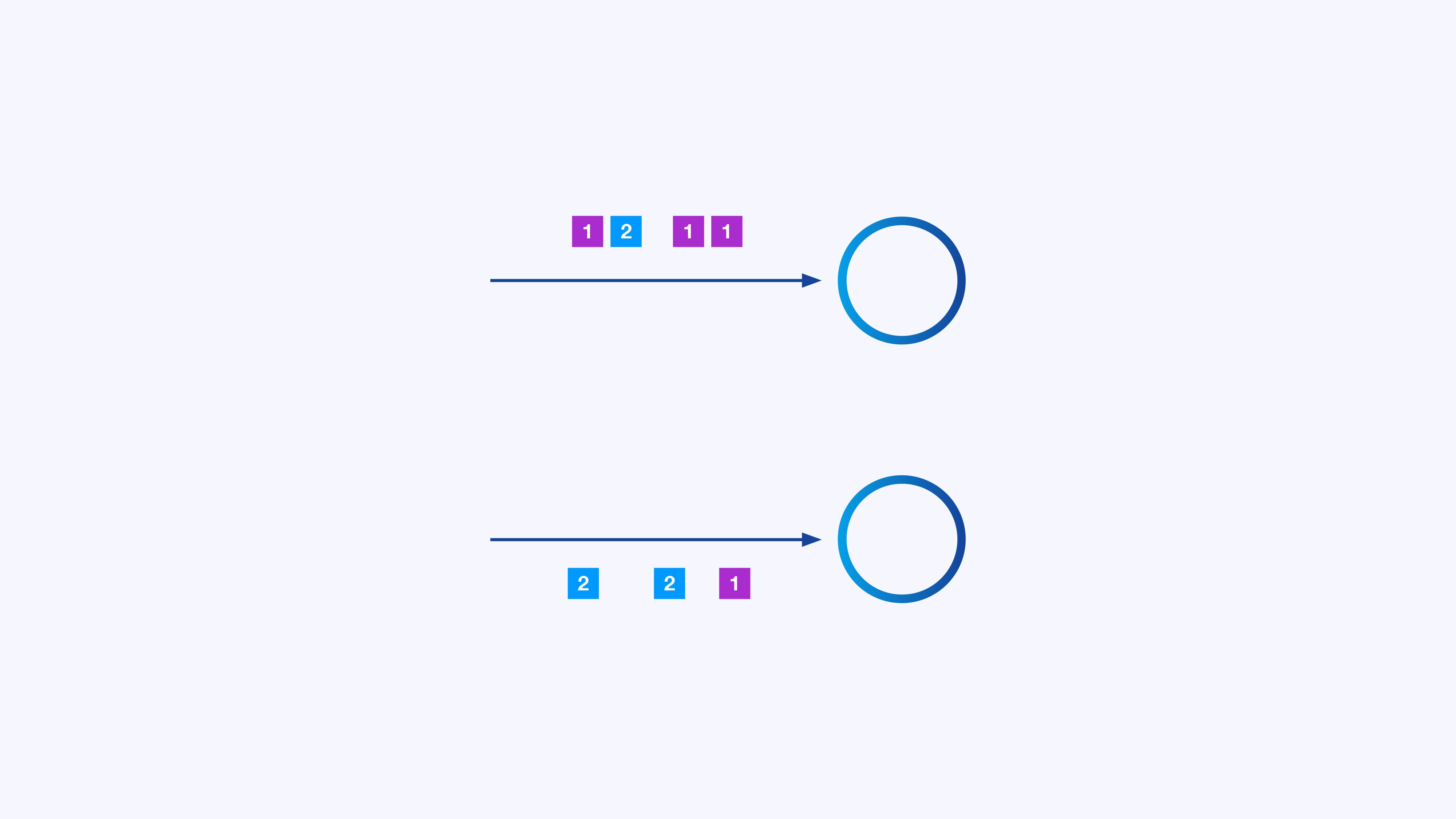
Each operator can have many parallel instances, each operating independently on some subset of the events.
IDG
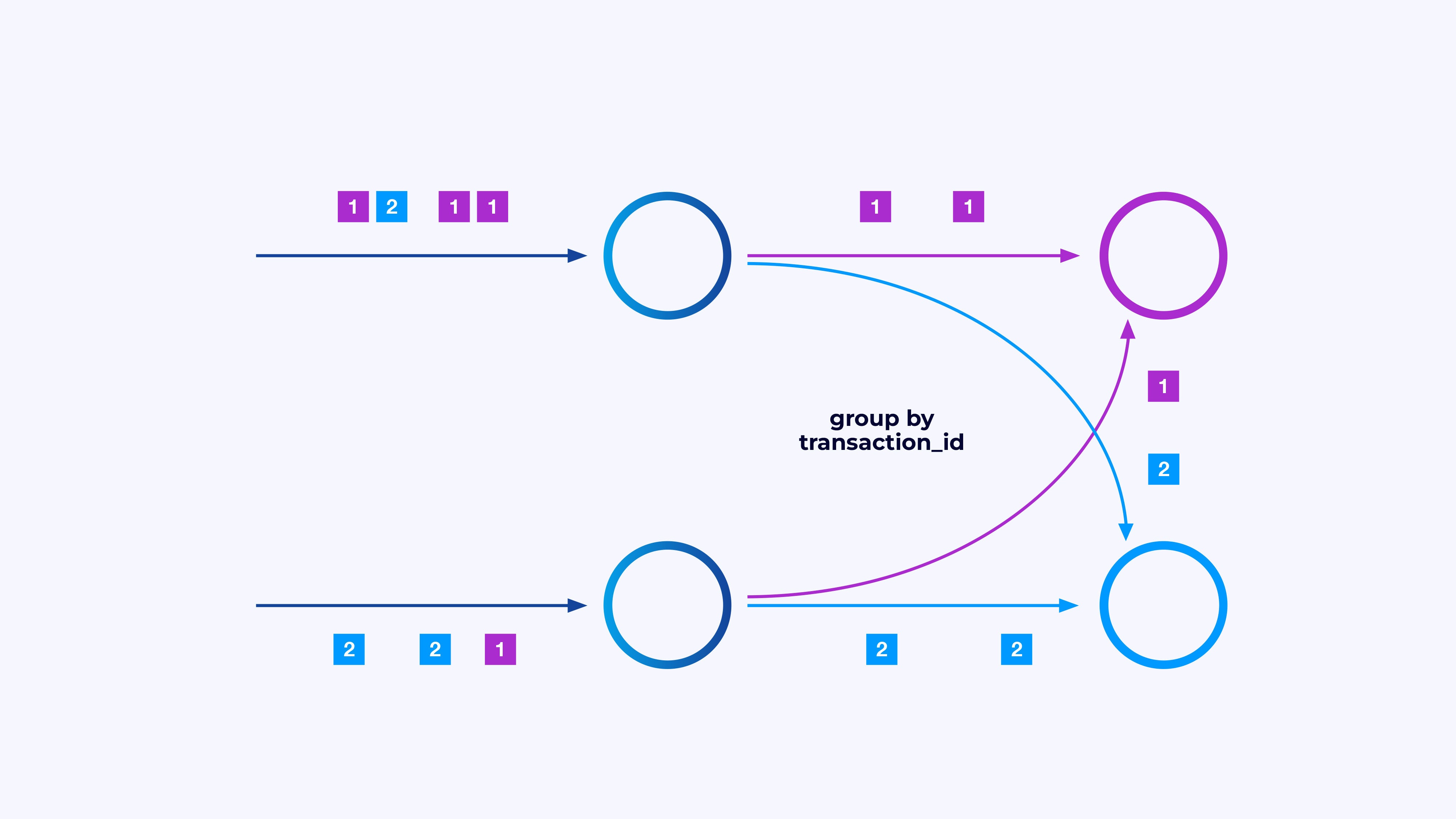
Sometimes you will want to impose a specific partitioning scheme on these sub-streams, so that the events are grouped together according to some application-specific logic. For example, if you’re processing financial transactions, you might want every event for any given transaction to be processed by the same thread. This will allow you to connect together the various events that occur over time for each transaction.
In Flink SQL you would do this with GROUP BY transaction_id, while in the DataStream API you would use keyBy(event -> event.transaction_id) to specify this grouping, or partitioning. In either case, this will show up in the job graph as a fully connected network shuffle between two consecutive stages of the graph.
IDG
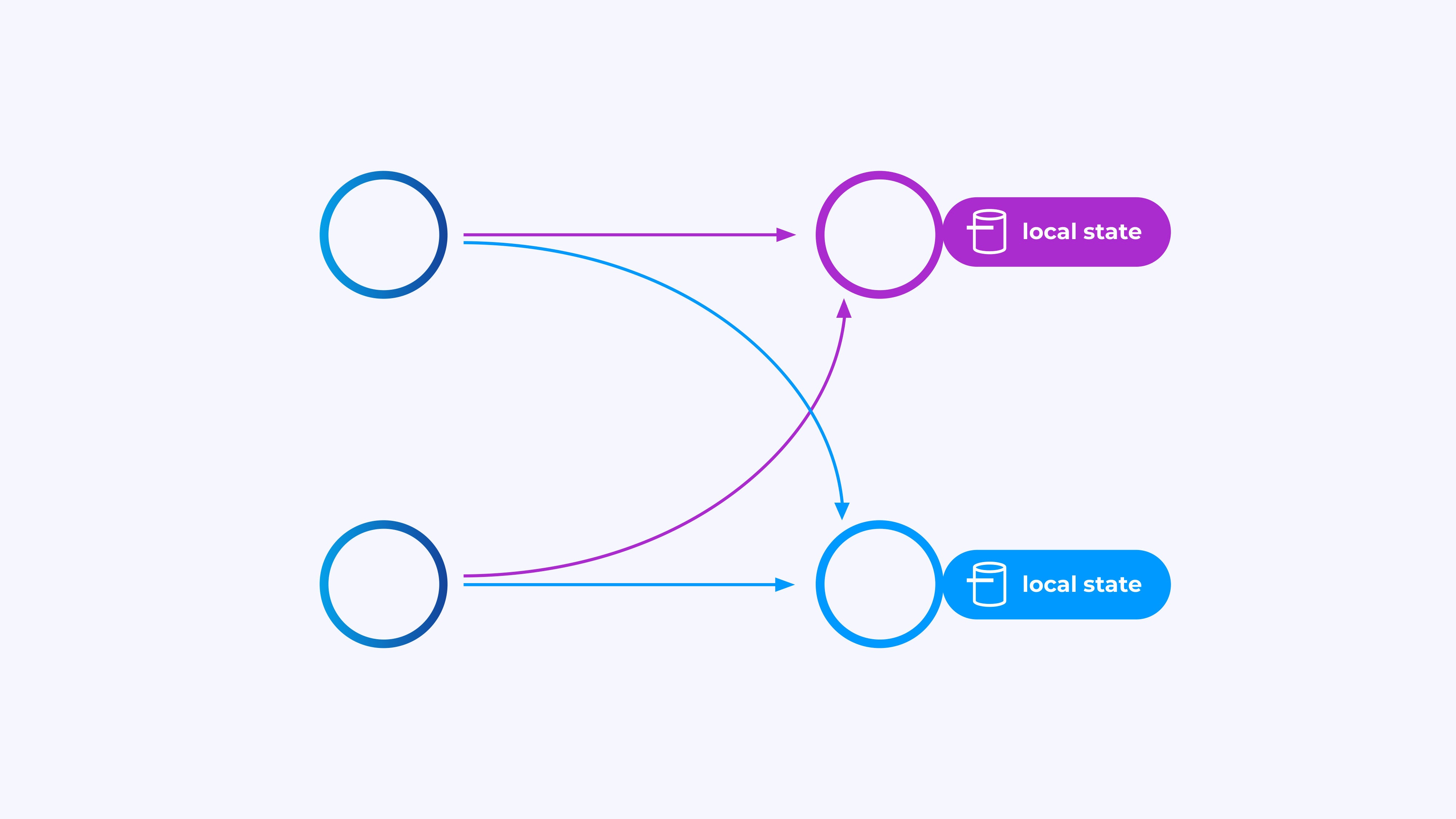
State
Operators working on key-partitioned streams can use Flink’s distributed key/value state store to durably persist whatever they want. The state for each key is local to a specific instance of an operator, and cannot be accessed from anywhere else. The parallel sub-topologies share nothing—this is crucial for unrestrained scalability.
IDG
A Flink job might be left running indefinitely. If a Flink job is continuously creating new keys (e.g., transaction IDs) and storing something for each new key, then that job risks blowing up because it is using an unbounded amount of state. Each of Flink’s APIs is organized around providing ways to help you avoid runaway explosions of state.
Time
One way to avoid hanging onto state for too long is to retain it only until some specific point in time. For instance, if you want to count transactions in minute-long windows, once each minute is over, the result for that minute can be produced, and that counter can be freed.
Flink makes an important distinction between two different notions of time:
Processing (or wall clock) time, which is derived from the actual time of day when an event is being processed.
Event time, which is based on timestamps recorded with each event.
To illustrate the difference between them, consider what it means for a minute-long window to be complete:
A processing time window is complete when the minute is over. This is perfectly straightforward.
An event time window is complete when all events that occurred during that minute have been processed. This can be tricky, since Flink can’t know anything about events it hasn’t processed yet. The best we can do is to make an assumption about how out-of-order a stream might be, and apply that assumption heuristically.
Checkpointing for failure recovery
Failures are inevitable. Despite failures, Flink is able to provide effectively exactly-once guarantees, meaning that each event will affect the state Flink is managing exactly once, just as though the failure never occurred. It does this by taking periodic, global, self-consistent snapshots of all the state. These snapshots, created and managed automatically by Flink, are called checkpoints.
Recovery involves rolling back to the state captured in the most recent checkpoint, and performing a global restart of all of the operators from that checkpoint. During recovery some events are reprocessed, but Flink is able to guarantee correctness by ensuring that each checkpoint is a global, self-consistent snapshot of the complete state of the system.
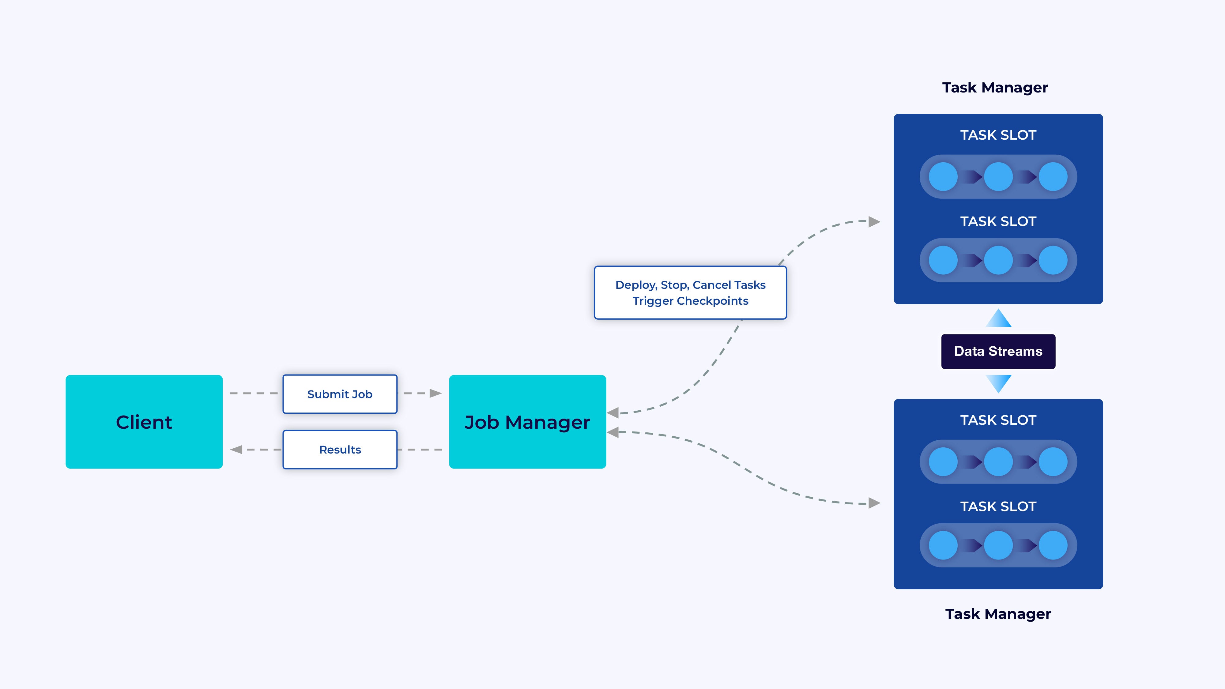
Flink system architecture
Flink applications run in Flink clusters, so before you can put a Flink application into production, you’ll need a cluster to deploy it to. Fortunately, during development and testing it’s easy to get started by running Flink locally in an integrated development environment like JetBrains IntelliJ, or in Docker.
A Flink cluster has two kinds of components: a job manager and a set of task managers. The task managers run your applications (in parallel), while the job manager acts as a gateway between the task managers and the outside world. Applications are submitted to the job manager, which manages the resources provided by the task managers, coordinates checkpointing, and provides visibility into the cluster in the form of metrics.
IDG
Flink developer experience
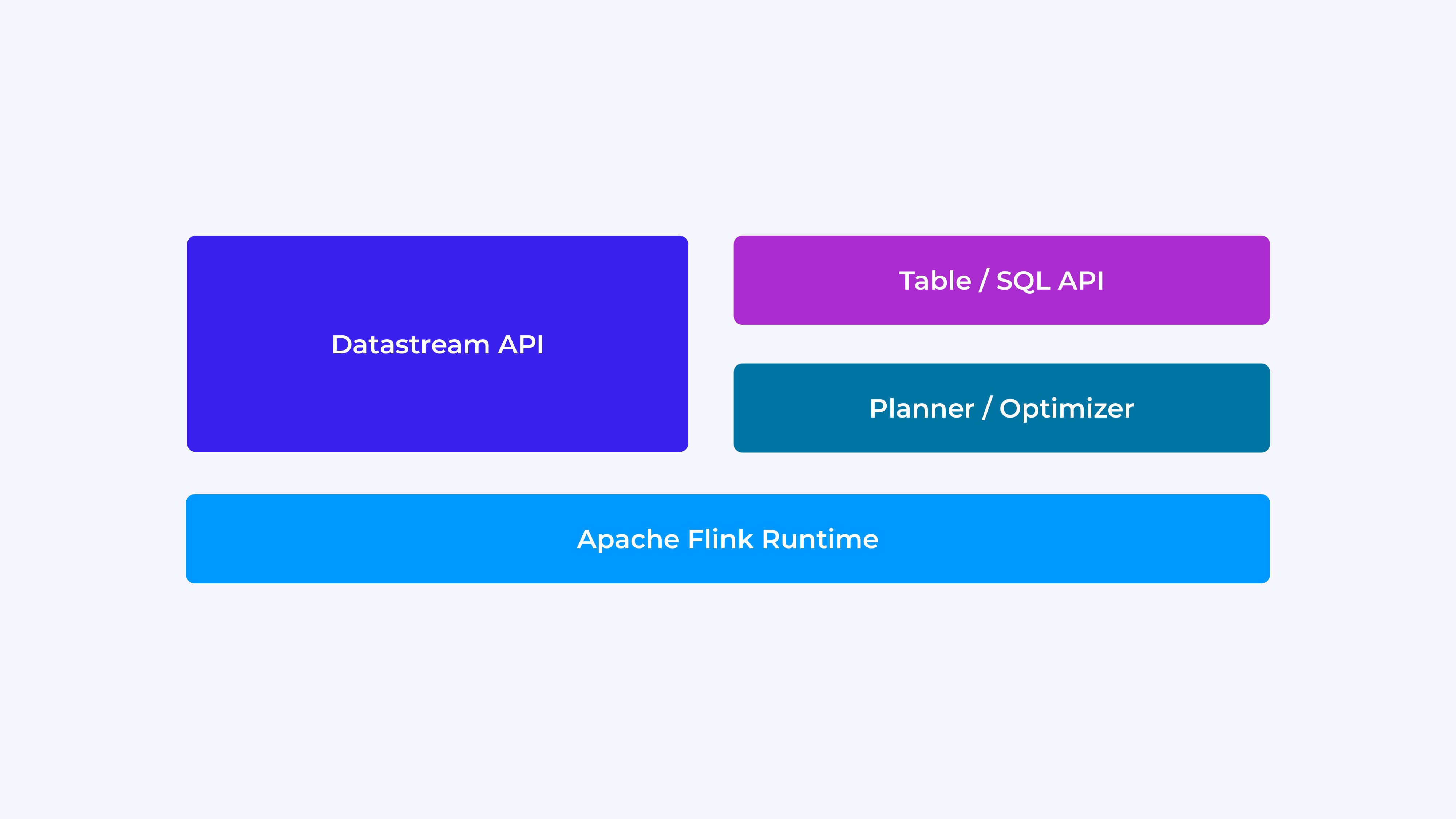
The experience you’ll have as a Flink developer depends, to a certain extent, on which of the APIs you choose: either the older, lower-level DataStream API or the newer, relational Table and SQL APIs.
IDG
When you are programming with Flink’s DataStream API, you are consciously thinking about what the Flink runtime will be doing as it runs your application. This means that you are building up the job graph one operator at a time, describing the state you are using along with the types involved and their serialization, creating timers and implementing callback functions to be executed when those timers are triggered, etc. The core abstraction in the DataStream API is the event, and the functions you write will be handling one event at a time, as they arrive.
On the other hand, when you use Flink’s Table/SQL API, these low-level concerns are taken care of for you, and you can focus more directly on your business logic. The core abstraction is the table, and you are thinking more in terms of joining tables for enrichment, grouping rows together to compute aggregated analytics, etc. A built-in SQL query planner/optimizer takes care of the details. The planner/optimizer does an excellent job of managing resources efficiently, often out-performing hand-written code.
A couple more thoughts before diving into the details: First, you don’t have to choose the DataStream or the Table/SQL API—both APIs are interoperable, and you can combine them. That can be a good way to go if you need a bit of customization that isn’t possible in the Table/SQL API. Second, another good way to go beyond what Table/SQL API offers out of the box is to add some additional capabilities in the form of user-defined functions (UDFs). Here, Flink SQL offers a lot of options for extension.
Constructing the job graph
Regardless of which API you use, the ultimate purpose of the code you write is to construct the job graph that Flink’s runtime will execute on your behalf. This means that these APIs are organized around creating operators and specifying both their behavior and their connections to one another. With the DataStream API you are directly constructing the job graph. With the Table/SQL API, Flink’s SQL planner is taking care of this.
Serializing functions and data
Ultimately, the code you supply to Flink will be executed in parallel by the workers (the task managers) in a Flink cluster. To make this happen, the function objects you create are serialized and sent to the task managers where they are executed. Similarly, the events themselves will sometimes need to be serialized and sent across the network from one task manager to another. Again, with the Table/SQL API you don’t have to think about this.
Managing state
The Flink runtime needs to be made aware of any state that you expect it to recover for you in the event of a failure. To make this work, Flink needs type information it can use to serialize and deserialize these objects (so they can be written into, and read from, checkpoints). You can optionally configure this managed state with time-to-live descriptors that Flink will then use to automatically expire state once it has outlived its usefulness.
With the DataStream API you generally end up directly managing the state your application needs (the built-in window operations are the one exception to this). On the other hand, with the Table/SQL API this concern is abstracted away. For example, given a query like the one below, you know that somewhere in the Flink runtime some data structure has to be maintaining a counter for each URL, but the details are all taken care of for you.
SELECT url, COUNT(*)
FROM pageviews
GROUP BY url;
Setting and triggering timers
Timers have many uses in stream processing. For example, it is common for Flink applications to need to gather information from many different event sources before eventually producing results. Timers work well for cases where it makes sense to wait (but not indefinitely) for data that may (or may not) eventually arrive.
Timers are also essential for implementing time-based windowing operations. Both the DataStream and Table/SQL APIs have built-in support for windows, and they are creating and managing timers on your behalf.
Flink use cases
Circling back to the three broad categories of streaming use cases introduced at the beginning of this article, let’s see how they map onto what you’ve just been learning about Flink.
Streaming data pipelines
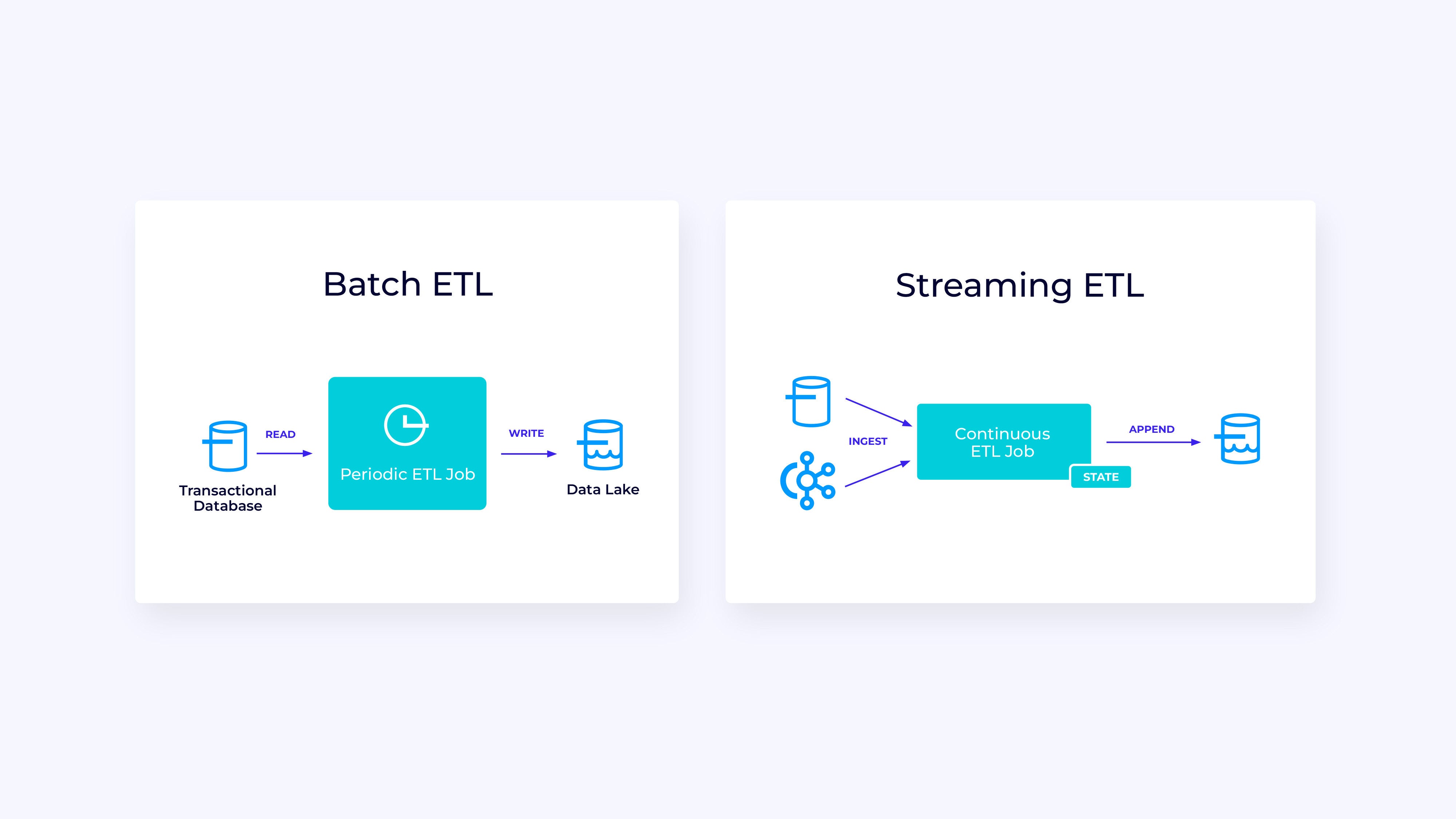
Below, at left, is an example of a traditional batch ETL (extract, transform, and load) job that periodically reads from a transactional database, transforms the data, and writes the results out to another data store, such as a database, file system, or data lake.
IDG
The corresponding streaming pipeline is superficially similar, but has some significant differences:
The streaming pipeline is always running.
The transactional data is being delivered to the streaming pipeline in two parts: an initial bulk load from the database and a change data capture (CDC) stream that delivers the database updates since that bulk load.
The streaming version continuously produces new results as soon as they become available.
State is explicitly managed so that it can be robustly recovered in the event of a failure. Streaming ETL pipelines typically use very little state. The data sources keep track of exactly how much of the input has been ingested, typically in the form of offsets that count records since the beginning of the streams. The sinks use transactions to manage their writes to external systems, like databases or Apache Kafka. During checkpointing, the sources record their offsets, and the sinks commit the transactions that carry the results of having read exactly up to, but not beyond, those source offsets.
For this use case, the Table/SQL API would be a good choice.
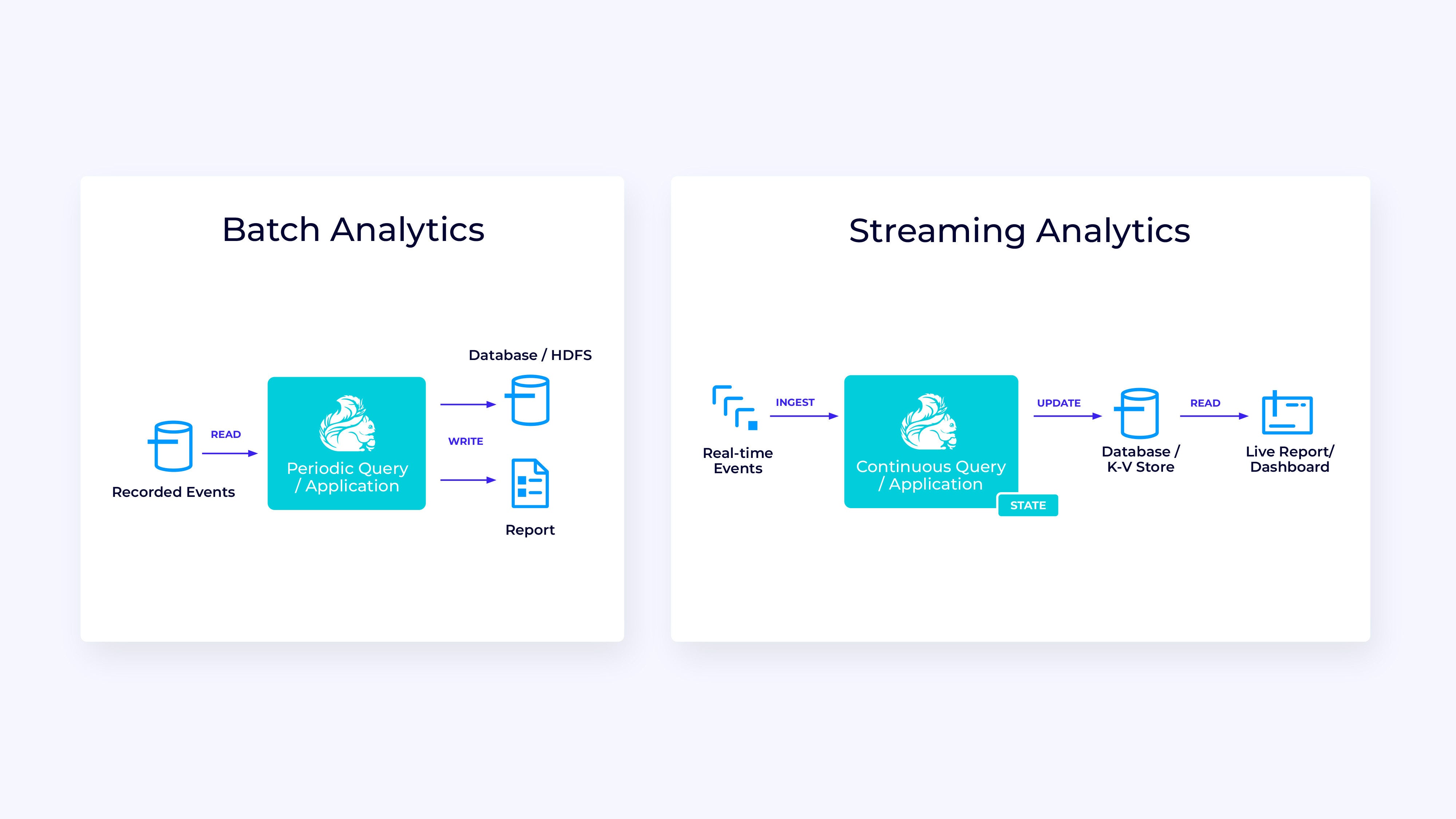
Real-time analytics
Compared to the streaming ETL application, the streaming analytics application has a couple of interesting differences:
As with streaming ETL, Flink is being used to run a continuous application, but for this application Flink will probably need to manage substantially more state.
For this use case it makes sense for the stream being ingested to be stored in a stream-native storage system, such as Kafka.
Rather than periodically producing a static report, the streaming version can be used to drive a live dashboard.
Once again, the Table/SQL API is usually a good choice for this use case.
IDG
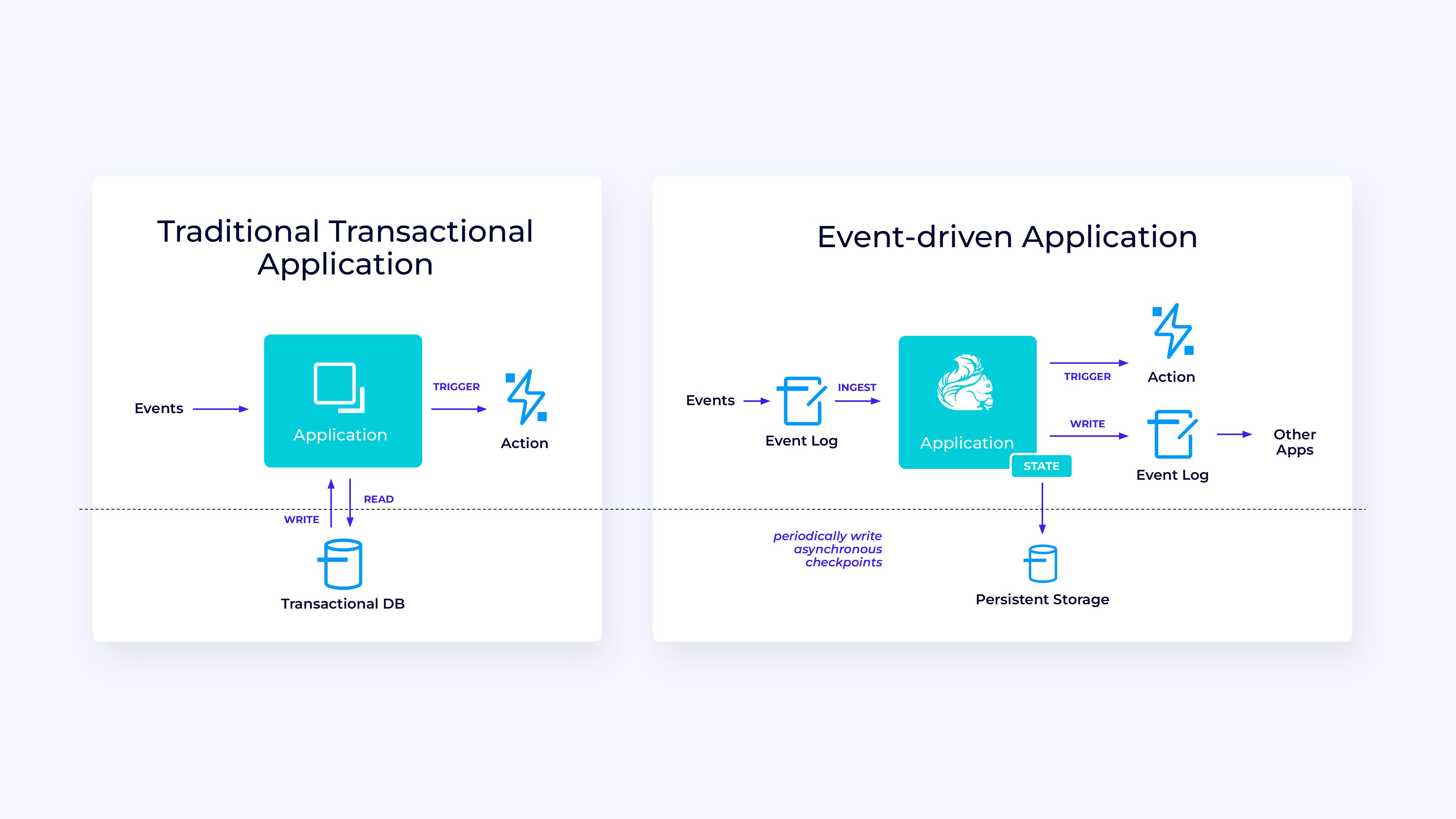
Event-driven applications
Our third and final family of use cases involves the implementation of event-driven applications or microservices. Much has been written on this topic; this is an architectural design pattern that has a lot of benefits.
IDG
Flink can be a great fit for these applications, especially if you need the kind of performance Flink can deliver. In some cases the Table/SQL API has everything you need, but in many cases you’ll need the additional flexibility of the DataStream API for at least part of the job.
Get started with Flink today
Flink provides a powerful framework for building applications that process event streams. Some of the concepts may seem novel at first, but once you’re familiar with the way Flink is designed and how it operates, the software is intuitive to use and the rewards of knowing Flink are significant.
As a next step, follow the instructions in the Flink documentation, which will guide you through the process of downloading, installing, and running the latest stable version of Flink. Think about the broad use cases we discussed—modern data pipelines, real-time analytics, and event-driven microservices—and how these can help to address a challenge or drive value for your organization.
Data streaming is one of the most exciting areas of enterprise technology today, and stream processing with Flink makes it even more powerful. Learning Flink will be beneficial for your organization, but also for your career, because real-time data processing is becoming more valuable to businesses globally. So check out Flink today and see what this powerful technology can help you achieve.
New Tech Forum provides a venue for technology leaders—including vendors and other outside contributors—to explore and discuss emerging enterprise technology in unprecedented depth and breadth. The selection is subjective, based on our pick of the technologies we believe to be important and of greatest interest to InfoWorld readers. InfoWorld does not accept marketing collateral for publication and reserves the right to edit all contributed content. Send all inquiries to doug_dineley@foundryco.com.
Spatiotemporal data, which comes from sources as diverse as cell phones, climate sensors, financial market transactions, and sensors in vehicles and containers, represents the largest and most rapidly expanding data category. IDC estimates that data generated from connected IoT devices will total 73.1 ZB by 2025, growing at a 26% CAGR from 18.3 ZB in 2019.
According to a recent report from MIT Technology Review Insights, IoT data (often tagged with location) is growing faster than other structured and semi-structured data (see figure below). Yet IoT data remains largely untapped by most organizations due to challenges associated with its complex integration and meaningful utilization.
The convergence of two groundbreaking technological advancements is poised to bring unprecedented efficiency and accessibility to the realms of geospatial and time-series data analysis. The first is GPU-accelerated databases, which bring previously unattainable levels of performance and precision to time-series and spatial workloads. The second is generative AI, which eliminates the need for individuals who possess both GIS expertise and advanced programming acumen.
These developments, both individually groundbreaking, have intertwined to democratize complex spatial and time-series analysis, making it accessible to a broader spectrum of data professionals than ever before. In this article, I explore how these advancements will reshape the landscape of spatiotemporal databases and usher in a new era of data-driven insights and innovation.
How the GPU accelerates spatiotemporal analysis
Originally designed to accelerate computer graphics and rendering, the GPU has recently driven innovation in other domains requiring massive parallel calculations, including the neural networks powering today’s most powerful generative AI models. Similarly, the complexity and range of spatiotemporal analysis has often been constrained by the scale of compute. But modern databases able to leverage GPU acceleration have unlocked new levels of performance to drive new insights. Here I will highlight two specific areas of spatiotemporal analysis accelerated by GPUs.
Inexact joins for time-series streams with different timestamps
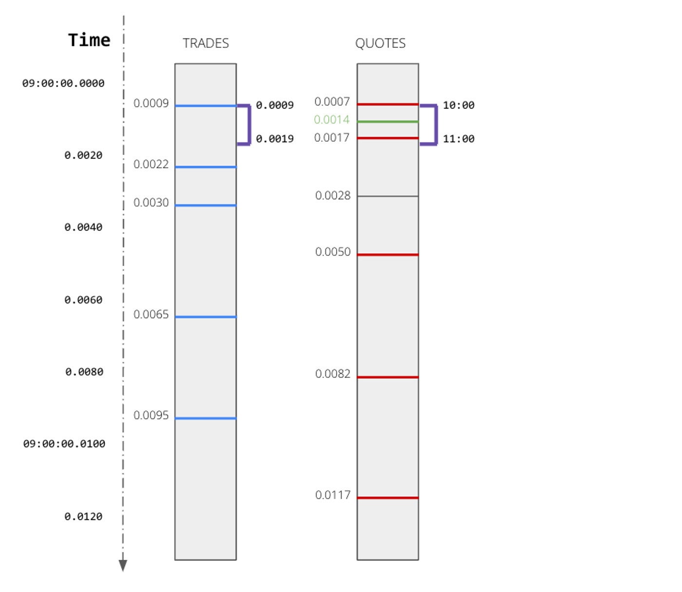
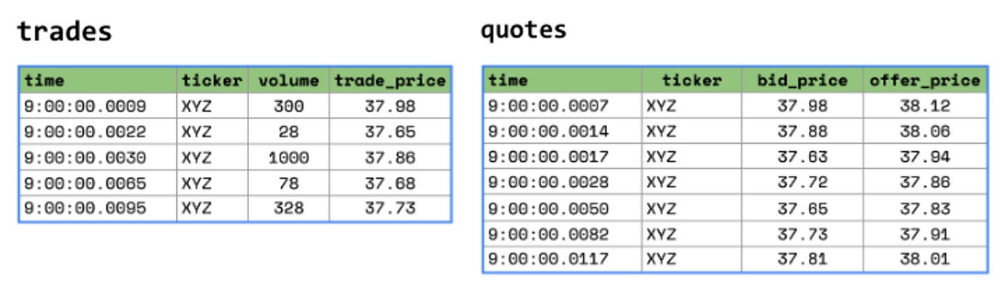
When analyzing disparate streams of time-series data, timestamps are rarely perfectly aligned. Even when devices rely on precise clocks or GPS, sensors may generate readings on different intervals or deliver metrics with different latencies. Or, in the case of stock trades and stock quotes, you may have interleaving timestamps that do not perfectly align.
To gain a common operational picture of the state of your machine data at any given time, you will need to join these different data sets (for instance, to understand the actual sensor values of your vehicles at any point along a route, or to reconcile financial trades against the most recent quotes). Unlike customer data, where you can join on a fixed customer ID, here you will need to perform an inexact join to correlate different streams based on time.
Rather than trying to build complicated data engineering pipelines to correlate time series, we can leverage the processing power of the GPU to do the heavy lifting. For instance, with Kinetica you can leverage the GPU accelerated ASOF join, which allows you to join one time-series dataset to another using a specified interval and whether the minimum or maximum value within that interval should be returned.
For instance, in the following scenario, trades and quotes arrive on different intervals.
IDG IDG
If I wanted to analyze Apple trades and their corresponding quotes, I could use Kinetica’s ASOF join to immediately find corresponding quotes that occurred within a certain interval of each Apple trade.
SELECT *
FROM trades t
LEFT JOIN quotes q
ON t.symbol = q.symbol
AND ASOF(t.time, q.timestamp, INTERVAL '0' SECOND, INTERVAL '5' SECOND, MIN)
WHERE t.symbol = 'AAPL'
There you have it. One line of SQL and the power of the GPU to replace the implementation cost and processing latency of complex data engineering pipelines for spatiotemporal data. This query will find for each trade the quote that was closest to that trade, within a window of five seconds after the trade. These types of inexact joins on time-series or spatial datasets are a critical tool to help harness the flood of spatiotemporal data.
Interactive geovisualization of billions of points
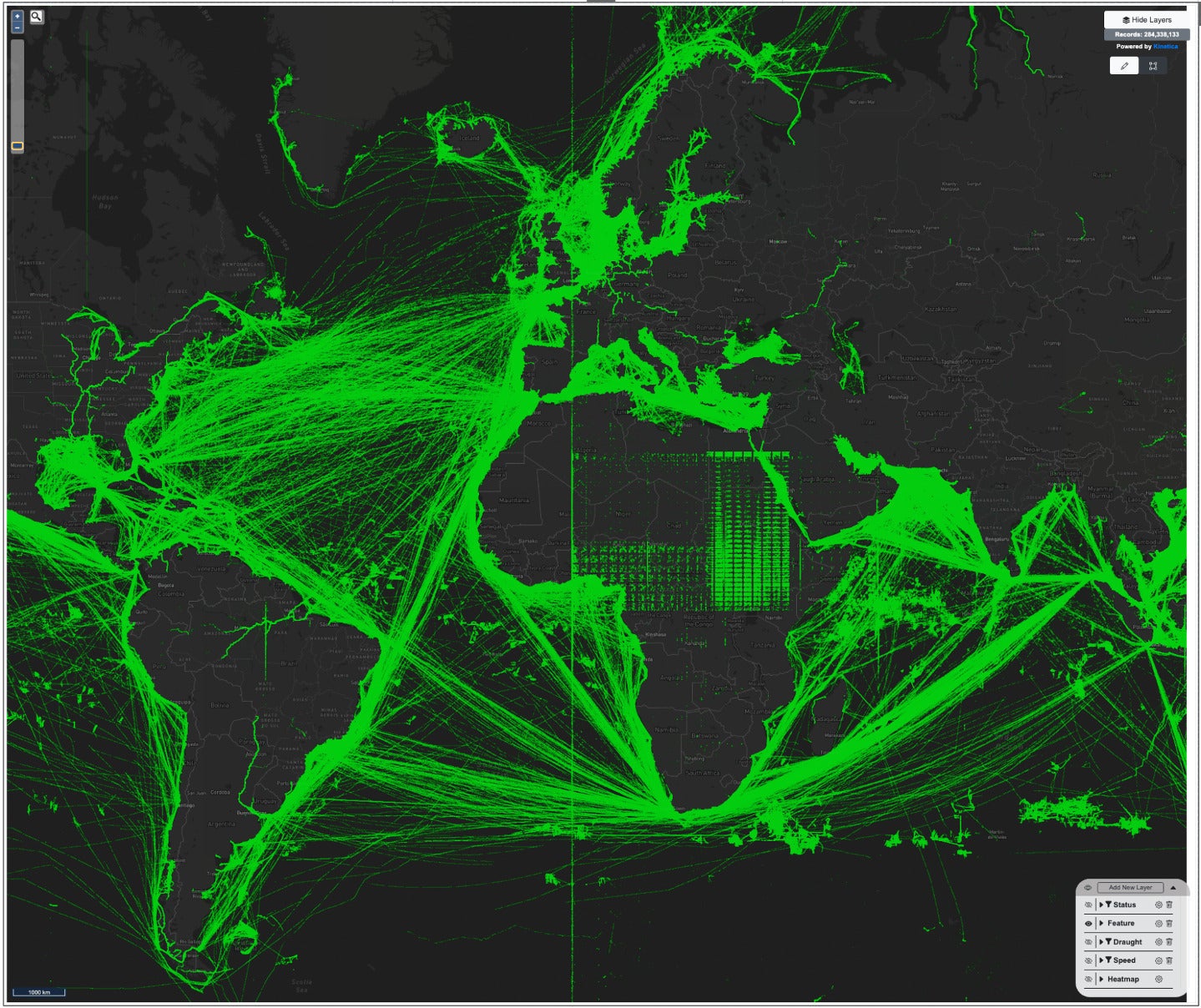
Often, the first step to exploring or analyzing spatiotemporal IoT data is visualization. Especially with geospatial data, rendering the data against a reference map will be the easiest way to perform a visual inspection of the data, checking for coverage issues, data quality issues, or other anomalies. For instance, it’s infinitely quicker to visually scan a map and confirm that your vehicles’ GPS tracks are actually following the road network versus developing other algorithms or processes to validate your GPS signal quality. Or, if you see spurious data around Null Island in the Gulf of Guinea, you can quickly identify and isolate invalid GPS data sources that are sending 0 degrees for latitude and 0 degrees for longitude.
However, analyzing large geospatial datasets at scale using conventional technologies often requires compromises. Conventional client-side rendering technologies typically can handle tens of thousands of points or geospatial features before rendering bogs down and the interactive exploration experience completely degrades. Exploring a subset of the data, for instance for a limited time window or a very limited geographic region, could reduce the volume of data to a more manageable quantity. However, as soon as you start sampling the data, you risk discarding data that would show specific data quality issues, trends, or anomalies that could have been easily discovered through visual analysis.
IDG
Visual inspection of nearly 300 million data points from shipping traffic can quickly reveal data quality issues, such as the anomalous data in Africa, or the band at the Prime Meridian.
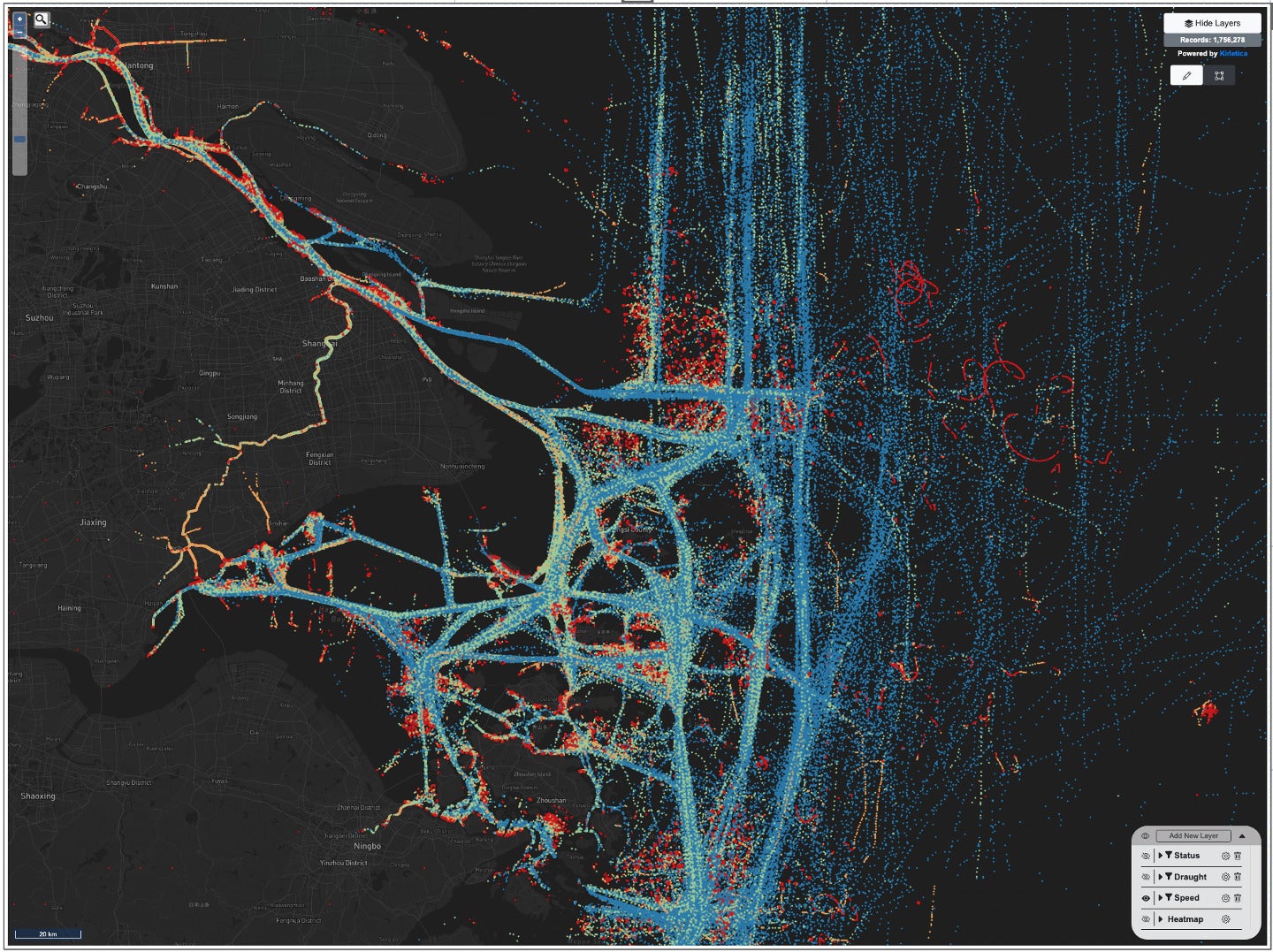
Fortunately, the GPU excels at accelerating visualizations. Modern database platforms with server-side GPU rendering capabilities such as Kinetica can facilitate exploration and visualization of millions or even billions of geospatial points and features in real time. This massive acceleration enables you to visualize all of your geospatial data instantly without downsampling, aggregation, or any reduction in data fidelity. The instant rendering provides a fluid visualization experience as you pan and zoom, encouraging exploration and discovery. Additional aggregations such as heat maps or binning can be selectively enabled to perform further analysis on the complete data corpus.
IDG
Zooming in to analyze shipping traffic patterns and vessel speed in the East China Sea.
Democratizing spatiotemporal analysis with LLMs
Spatiotemporal questions, which pertain to the relationship between space and time in data, often resonate intuitively with laymen because they mirror real-world experiences. People might wonder about the journey of an item from the moment of order placement to its successful delivery. However, translating these seemingly straightforward inquiries into functional code poses a formidable challenge, even for seasoned programmers.
For instance, determining the optimal route for a delivery truck that minimizes travel time while factoring in traffic conditions, road closures, and delivery windows requires intricate algorithms and real-time data integration. Similarly, tracking the spread of a disease through both time and geography, considering various influencing factors, demands complex modeling and analysis that can baffle even experienced data scientists.
These examples highlight how spatio-temporal questions, though conceptually accessible, often hide layers of complexity that make their coding a daunting task. Understanding the optimal mathematical operations and then the corresponding SQL function syntax may challenge even the most seasoned SQL experts.
Thankfully, the latest generation of large language models (LLMs) are proficient at generating correct and efficient code, including SQL. And fine-tuned versions of those models that have been trained on the nuances of spatiotemporal analysis, such as Kinetica’s native LLM for SQL-GPT, can now unlock these domains of analysis for a whole new class of users.
For instance, let’s say I wanted to analyze the canonical New York City taxi data set and pose questions related to space and time. I start by providing the LLM with some basic context about the tables I intend to analyze. In Kinetica Cloud, I can use the UI or basic SQL commands to define the context for my analysis, including references to the specific tables. The column names and definitions for those tables are shared with the LLM, but not any data from those tables. Optionally, I can include additional comments, rules, or sample query results in the context to further improve the accuracy of my SQL.
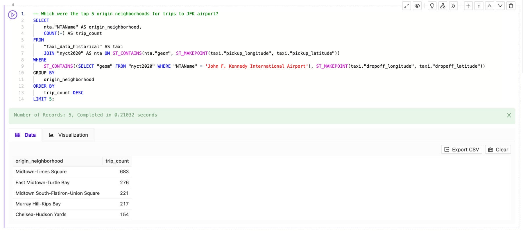
Once I have set up the initial context, I can use SQL-GPT in Kinetica Cloud to ask “Which were the top 5 origin neighborhoods for trips to JFK airport?” The fine-tuned LLM instantly generates the following SQL:
-- Which were the top 5 origin neighborhoods for trips to JFK airport?
SELECT
nta."NTAName" AS origin_neighborhood,
COUNT(*) AS trip_count
FROM
"taxi_data_historical" AS taxi
JOIN   "nyct2020" AS nta
ON     ST_CONTAINS(nta."geom", ST_MAKEPOINT(taxi."pickup_longitude", taxi."pickup_latitude"))
WHERE ST_CONTAINS((
            SELECT "geom"
            FROM "nyct2020"
            WHERE "NTAName" = 'John F. Kennedy International Airport'
            ),
            ST_MAKEPOINT(taxi."dropoff_longitude", taxi."dropoff_latitude"))
GROUP BY
origin_neighborhood
ORDER BY
trip_count DESC
LIMIT 5;
Within seconds, the fine-tuned LLM helped me to:
Set up the SELECT statement, referencing the right target tables and columns, setting up the JOIN and using COUNT(*), GROUP BY, ORDER BY, and LIMIT. For those less proficient in SQL, even that basic query construction is a tremendous accelerant.
Utilize the correct spatial functions, such as ST_MAKEPOINT() to create a point from a latitude and longitude and ST_CONTAINS() to find geographic areas that contain the specified point. By helping me to choose the right functions and syntax, the LLM can help jump-start spatial analysis for those new to the field.
Integrate real-world references to locations and times. I asked about “JFK airport” but the LLM was able to translate this reference into the Neighborhood Tabulation Area named “John F. Kennedy International Airport.” Another time-saver—thanks, LLM!
Now I run the query to answer my initial question:
IDG
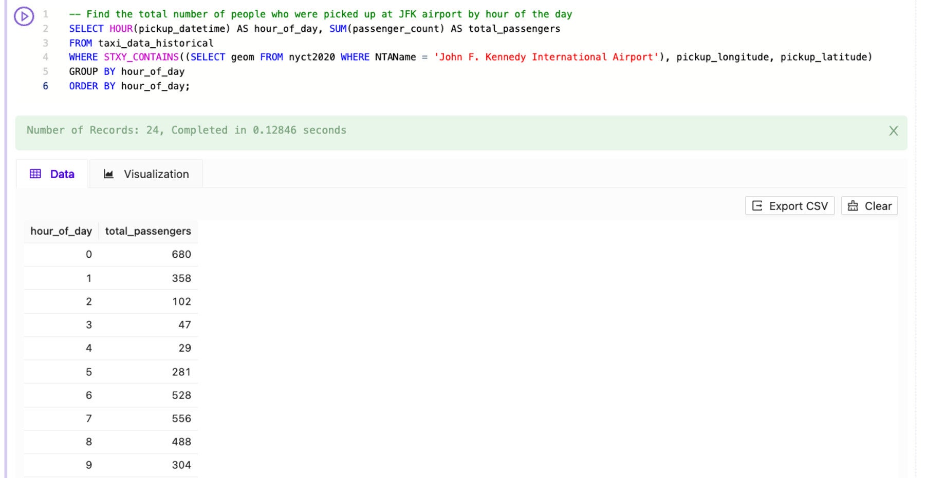
Similarly, if I ask Kinetica SQL-GPT to help me “Find the total number of people who were picked up at JFK airport by hour of the day,” it generates the following SQL:
-- Find the total number of people who were picked up at JFK airport by hour of the day
SELECT HOUR(pickup_datetime) AS hour_of_day, SUM(passenger_count) AS total_passengers
FROM taxi_data_historical
WHERE STXY_CONTAINS((SELECT geom FROM nyct2020 WHERE NTAName = 'John F. Kennedy International Airport'), pickup_longitude, pickup_latitude)
GROUP BY hour_of_day
ORDER BY hour_of_day;
This query incorporated additional complexity around summing the number of passengers in each taxi and bucketing the data by hour of day. But the LLM handled the complexity and instantly generated proper SQL.
IDG
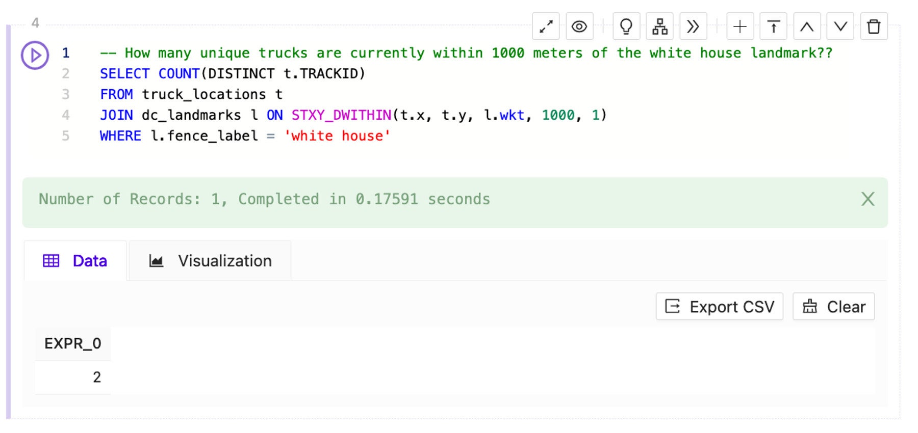
For more sophisticated users, the LLM can also handle more advanced spatiotemporal processing. For instance, in the next example, I would like to analyze a fleet of trucks out for deliveries in the Washington DC area and I want to understand which trucks are currently close to a set of geofences (in this case, buffers around famous DC landmarks).
I could start with a basic question around proximity to a specific geofence, such as “How many unique trucks are currently within 1000 meters of the white house landmark?” and use Kinetica SQL-GPT to generate the following SQL:
-- How many unique trucks are currently within 1000 meters of the white house landmark?
SELECT COUNT(DISTINCT r.TRACKID)
FROM recent_locations r
JOIN dc_landmarks d ON STXY_DWITHIN(r.x, r.y, d.wkt, 1000, 1)
WHERE d.fence_label = 'white house'
IDG
But if I want to have a constantly refreshing view of which trucks are near my geofences, I can get the LLM to help me create a materialized view.
Starting with the prompt “Which trucks came within 200 meters of a landmark in Washington DC in the last 5 mins? Keep all the columns and create a materialized view called landmark_trucks that refreshes every 10 seconds to store the results,” Kinetica SQL-GPT and the LLM are able to generate the SQL to create and refresh the materialized view:
-- Which trucks came within 200 meters of a landmark in Washington DC in the last 5 mins? Keep all the columns and create a materialized view called landmark_trucks that refreshes every 10 seconds to store the results.
CREATE OR REPLACE MATERIALIZED VIEW landmark_trucks REFRESH EVERY 10 SECONDS AS
SELECT *
FROM truck_locations t
JOIN dc_landmarks d ON STXY_DWITHIN(t.x, t.y, d.wkt, 200, 1)
WHERE t."TIMESTAMP" >= NOW() - INTERVAL '5' MINUTE;
To harness the ever-increasing volume of spatiotemporal data, enterprises will need to modernize their data platforms to handle the scale of analysis and deliver the insights and optimizations their business depends on. Fortunately, recent advancements in GPUs and generative AI are ready to transform the world of spatiotemporal analysis.
GPU accelerated databases dramatically simplify the processing and exploration of spatiotemporal data at scale. With the latest advancements in large language models that are fine-tuned for natural language to SQL, the techniques of spatiotemporal analysis can be democratized further in the organization, beyond the traditional domains of GIS analysts and SQL experts. The rapid innovation in GPUs and generative AI will surely make this an exciting space to watch.
Philip Darringer is vice president of product management for Kinetica, where he guides the development of the company’s real-time, analytic database for time series and spatiotemporal workloads. He has more than 15 years of experience in enterprise product management with a focus on data analytics, machine learning, and location intelligence.
—
Generative AI Insights provides a venue for technology leaders to explore and discuss the challenges and opportunities of generative artificial intelligence. The selection is wide-ranging, from technology deep dives to case studies to expert opinion, but also subjective, based on our judgment of which topics and treatments will best serve InfoWorld’s technically sophisticated audience. InfoWorld does not accept marketing collateral for publication and reserves the right to edit all contributed content. Contact doug_dineley@foundryco.com.
When the leaves fall, the sky turns gray, the cold begins to bite, and we’re all yearning for a little sunshine, you know it’s time for InfoWorld’s Best of Open Source Software Awards, a fall ritual we affectionately call the Bossies. For 17 years now, the Bossies have celebrated the best and most innovative open source software.
As in years past, our top picks for 2023 include an amazingly eclectic mix of technologies. Among the 25 winners you’ll find programming languages, runtimes, app frameworks, databases, analytics engines, machine learning libraries, large language models (LLMs), tools for deploying LLMs, and one or two projects that beggar description.
If there is an important problem to be solved in software, you can bet that an open source project will emerge to solve it. Read on to meet our 2023 Bossies.
Apache Hudi
When building an open data lake or data lakehouse, many industries require a more evolvable and mutable platform. Take ad platforms for publishers, advertisers, and media buyers. Fast analytics aren’t enough. Apache Hudi not only provides a fast data format, tables, and SQL but also enables them for low-latency, real-time analytics. It integrates with Apache Spark, Apache Flink, and tools like Presto, StarRocks (see below), and Amazon Athena. In short, if you’re looking for real-time analytics on the data lake, Hudi is a really good bet.
— Andrew C. Oliver
Apache Iceberg
Who cares if something “scales well” if the result takes forever? HDFS and Hive were just too damn slow. Enter Apache Iceberg, which works with Hive, but also directly with Apache Spark and Apache Flink, as well as other systems like ClickHouse, Dremio, and StarRocks. Iceberg provides a high-performance table format for all of these systems while enabling full schema evolution, data compaction, and version rollback. Iceberg is a key component of many modern open data lakes.
— Andrew C. Oliver
Apache Superset
For many years, Apache Superset has been a monster of data visualization. Superset is practically the only choice for anyone wanting to deploy self-serve, customer-facing, or user-facing analytics at scale. Superset provides visualization for virtually any analytics scenario, including everything from pie charts to complex geospatial charts. It speaks to most SQL databases and provides a drag-and-drop builder as well as a SQL IDE. If you’re going to visualize data, Superset deserves your first look.
— Andrew C. Oliver
Bun
Just when you thought JavaScript was settling into a predictable routine, along comes Bun. The frivolous name belies a serious aim: Put everything you need for server-side JS—runtime, bundler, package manager—in one tool. Make it a drop-in replacement for Node.js and NPM, but radically faster. This simple proposition seems to have made Bun the most disruptive bit of JavaScript since Node flipped over the applecart.
Bun owes some of its speed to Zig (see below); the rest it owes to founder Jared Sumner’s obsession with performance. You can feel the difference immediately on the command line. Beyond performance, just having all of the tools in one integrated package makes Bun a compelling alternative to Node and Deno.
— Matthew Tyson
Claude 2
Anthropic’s Claude 2 accepts up to 100K tokens (about 70,000 words) in a single prompt, and can generate stories up to a few thousand tokens. Claude can edit, rewrite, summarize, classify, extract structured data, do Q&A based on the content, and more. It has the most training in English, but also performs well in a range of other common languages. Claude also has extensive knowledge of common programming languages.
Claude was constitutionally trained to be helpful, honest, and harmless (HHH), and extensively red-teamed to be more harmless and harder to prompt to produce offensive or dangerous output. It doesn’t train on your data or consult the internet for answers. Claude is available to users in the US and UK as a free beta, and has been adopted by commercial partners such as Jasper, Sourcegraph, and AWS.
— Martin Heller
CockroachDB
A distributed SQL database that enables strongly consistent ACID transactions, CockroachDB solves a key scalability problem for high-performance, transaction-heavy applications by enabling horizontal scalability of database reads and writes. CockroachDB also supports multi-region and multi-cloud deployments to reduce latency and comply with data regulations. Example deployments include Netflix’s Data Platform, with more than 100 production CockroachDB clusters supporting media applications and device management. Marquee customers also include Hard Rock Sportsbook, JPMorgan Chase, Santander, and DoorDash.
— Isaac Sacolick
CPython
Machine learning, data science, task automation, web development… there are countless reasons to love the Python programming language. Alas, runtime performance is not one of them—but that’s changing. In the last two releases, Python 3.11 and Python 3.12, the core Python development team has unveiled a slew of transformative upgrades to CPython, the reference implementation of the Python interpreter. The result is a Python runtime that’s faster for everyone, not just for the few who opt into using new libraries or cutting-edge syntax. And the stage has been set for even greater improvements with plans to remove the Global Interpreter Lock, a longtime hindrance to true multi-threaded parallelism in Python.
— Serdar Yegulalp
DuckDB
OLAP databases are supposed to be huge, right? Nobody would describe IBM Cognos, Oracle OLAP, SAP Business Warehouse, or ClickHouse as “lightweight.” But what if you needed just enough OLAP—an analytics database that runs embedded, in-process, with no external dependencies? DuckDB is an analytics database built in the spirit of tiny-but-powerful projects like SQLite. DuckDB offers all the familiar RDBMS features—SQL queries, ACID transactions, secondary indexes—but adds analytics features like joins and aggregates over large datasets. It can also ingest and directly query common big data formats like Parquet.
— Serdar Yegulalp
HTMX and Hyperscript
You probably thought HTML would never change. HTMX takes the HTML you know and love and extends it with enhancements that make it easier to write modern web applications. HTMX eliminates much of the boilerplate JavaScript used to connect web front ends to back ends. Instead, it uses intuitive HTML properties to perform tasks like issuing AJAX requests and populating elements with data. A sibling project, Hyperscript, introduces a HyperCard-like syntax to simplify many JavaScript tasks including asynchronous operations and DOM manipulations. Taken together, HTMX and Hyperscript offer a bold alternative vision to the current trend in reactive frameworks.
— Matthew Tyson
Istio
Simplifying networking and communications for container-based microservices, Istio is a service mesh that provides traffic routing, monitoring, logging, and observability while enhancing security with encryption, authentication, and authorization capabilities. Istio separates communications and their security functions from the application and infrastructure, enabling a more secure and consistent configuration. The architecture consists of a control plane deployed in Kubernetes clusters and a data plane for controlling communication policies. In 2023, Istio graduated from CNCF incubation with significant traction in the cloud-native community, including backing and contributions from Google, IBM, Red Hat, Solo.io, and others.
— Isaac Sacolick
Kata Containers
Combining the speed of containers and the isolation of virtual machines, Kata Containers is a secure container runtime that uses Intel Clear Containers with Hyper.sh runV, a hypervisor-based runtime. Kata Containers works with Kubernetes and Docker while supporting multiple hardware architectures including x86_64, AMD64, Arm, IBM p-series, and IBM z-series. Google Cloud, Microsoft, AWS, and Alibaba Cloud are infrastructure sponsors. Other companies supporting Kata Containers include Cisco, Dell, Intel, Red Hat, SUSE, and Ubuntu. A recent release brought confidential containers to GPU devices and abstraction of device management.
— Isaac Sacolick
LangChain
LangChain is a modular framework that eases the development of applications powered by language models. LangChain enables language models to connect to sources of data and to interact with their environments. LangChain components are modular abstractions and collections of implementations of the abstractions. LangChain off-the-shelf chains are structured assemblies of components for accomplishing specific higher-level tasks. You can use components to customize existing chains and to build new chains. There are currently three versions of LangChain: One in Python, one in TypeScript/JavaScript, and one in Go. There are roughly 160 LangChain integrations as of this writing.
— Martin Heller
Language Model Evaluation Harness
When a new large language model (LLM) is released, you’ll typically see a brace of evaluation scores comparing the model with, say, ChatGPT on a certain benchmark. More likely than not, the company behind the model will have used lm-eval-harness to generate those scores. Created by EleutherAI, the distributed artificial intelligence research institute, lm-eval-harness contains over 200 benchmarks, and it’s easily extendable. The harness has even been used to discover deficiencies in existing benchmarks, as well as to power Hugging Face’s Open LLM Leaderboard. Like in the xkcd cartoon, it’s one of those little pillars holding up an entire world.
— Ian Pointer
Llama 2
Llama 2 is the next generation of Meta AI’s large language model, trained on 40% more data (2 trillion tokens from publicly available sources) than Llama 1 and having double the context length (4096). Llama 2 is an auto-regressive language model that uses an optimized transformer architecture. The tuned versions use supervised fine-tuning (SFT) and reinforcement learning with human feedback (RLHF) to align to human preferences for helpfulness and safety. Code Llama, which was trained by fine-tuning Llama 2 on code-specific datasets, can generate code and natural language about code from code or natural language prompts.
— Martin Heller
Ollama
Ollama is a command-line utility that can run Llama 2, Code Llama, and other models locally on macOS and Linux, with Windows support planned. Ollama currently supports almost two dozen families of language models, with many “tags” available for each model family. Tags are variants of the models trained at different sizes using different fine-tuning and quantized at different levels to run well locally. The higher the quantization level, the more accurate the model is, but the slower it runs and the more memory it requires.
The models Ollama supports include some uncensored variants. These are built using a procedure devised by Eric Hartford to train models without the usual guardrails. For example, if you ask Llama 2 how to make gunpowder, it will warn you that making explosives is illegal and dangerous. If you ask an uncensored Llama 2 model the same question, it will just tell you.
— Martin Heller
Polars
You might ask why Python needs another dataframe-wrangling library when we already have the venerable Pandas. But take a deeper look, and you might find Polars to be exactly what you’re looking for. Polars can’t do everything Pandas can do, but what it can do, it does fast—up to 10x faster than Pandas, using half the memory. Developers coming from PySpark will feel a little more at home with the Polars API than with the more esoteric operations in Pandas. If you’re working with large amounts of data, Polars will allow you to work faster.
Tim Dettmers and team seem on a mission to make large language models run on everything down to your toaster. Last year, their bitsandbytes library brought inference of larger LLMs to consumer hardware. This year, they’ve turned to training, shrinking down the already impressive LoRA techniques to work on quantized models. Using QLoRA means you can fine-tune massive 30B-plus parameter models on desktop machines, with little loss in accuracy compared to full tuning across multiple GPUs. In fact, sometimes QLoRA does even better. Low-bit inference and training mean that LLMs are accessible to even more people—and isn’t that what open source is all about?
— Ian Pointer
RAPIDS
RAPIDS is a collection of GPU-accelerated libraries for common data science and analytics tasks. Each library handles a specific task, like cuDF for dataframe processing, cuGraph for graph analytics, and cuML for machine learning. Other libraries cover image processing, signal processing, and spatial analytics, while integrations bring RAPIDS to Apache Spark, SQL, and other workloads. If none of the existing libraries fits the bill, RAPIDS also includes RAFT, a collection of GPU-accelerated primitives for building one’s own solutions. RAPIDS also works hand-in-hand with Dask to scale across multiple nodes, and with Slurm to run in high-performance computing environments.
Spark NLP is a natural language processing library that runs on Apache Spark with Python, Scala, and Java support. The library helps developers and data scientists experiment with large language models including transformer models from Google, Meta, OpenAI, and others. Spark NLP’s model hub has more than 20 thousand models and pipelines to download for language translation, named entity recognition, text classification, question answering, sentiment analysis, and other use cases. In 2023, Spark NLP released many LLM integrations, a new image-to-text annotator designed for captioning images, support for all major public cloud storage systems, and ONNX (Open Neural Network Exchange) support.
— Isaac Sacolick
StarRocks
Analytics has changed. Companies today often serve complex data to millions of concurrent users in real time. Even petabyte queries must be served in seconds. StarRocks is a query engine that combines native code (C++), an efficient cost-based optimizer, vector processing using the SIMD instruction set, caching, and materialized views to efficiently handle joins at scale. StarRocks even provides near-native performance when directly querying from data lakes and data lakehouses including Apache Hudi and Apache Iceberg. Whether you’re pursuing real-time analytics, serving customer-facing analytics, or just wanting to query your data lake without moving data around, StarRocks deserves a look.
— Ian Pointer
TensorFlow.js
TensorFlow.js packs the power of Google’s TensorFlow machine learning framework into a JavaScript package, bringing extraordinary capabilities to JavaScript developers with a minimal learning curve. You can run TensorFlow.js in the browser, on a pure JavaScript stack with WebGL acceleration, or against the tfjs-node library on the server. The Node library gives you the same JavaScript API but runs atop the C binary for maximum speed and CPU/GPU usage.
If you are a JS developer interested in machine learning, TensorFlow.js is an obvious place to go. It’s a welcome contribution to the JS ecosystem that brings AI into easier reach of a broad community of developers.
— Matthew Tyson
vLLM
The rush to deploy large language models in production has resulted in a surge of frameworks focused on making inference as fast as possible. vLLM is one of the most promising, coming complete with Hugging Face model support, an OpenAI-compatible API, and PagedAttention, an algorithm that achieves up to 20x the throughput of Hugging Face’s transformers library. It’s one of the clear choices for serving LLMs in production today, and new features like FlashAttention 2 support are being added quickly.
— Ian Pointer
Weaviate
The generative AI boom has sparked the need for a new breed of database that can support massive amounts of complex, unstructured data. Enter the vector database. Weaviate offers developers loads of flexibility when it comes to deployment model, ecosystem integration, and data privacy. Weaviate combines keyword search with vector search for fast, scalable discovery of multimodal data (think text, images, audio, video). It also has out-of-the-box modules for retrieval-augmented generation (RAG), which provides chatbots and other generative AI apps with domain-specific data to make them more useful.
— Andrew C. Oliver
Zig
Of all the open-source projects going today, Zig may be the most momentous. Zig is an effort to create a general-purpose programming language with program-level memory controls that outperforms C, while offering a more powerful and less error-prone syntax. The goal is nothing less than supplanting C as the baseline language of the programming ecosystem. Because C is ubiquitous (i.e., the most common component in systems and devices everywhere), success for Zig could mean widespread improvements in performance and stability. That’s something we should all hope for. Plus, Zig is a good, old-fashioned grass-roots project with a huge ambition and an open-source ethos.